The Problem
You want a sampler for p_{\text{data}}(x). GANs play a minimax game that often diverges. VAEs produce blurry samples from a Gaussian decoder. What you really want is a training objective that is (a) a single stable loss (no saddle point, no minimax), (b) a lower bound on \log p(x) (so you have likelihoods), and (c) samples that match SOTA quality.
Sohl-Dickstein et al. (2015) had a theoretical answer: define a Markov chain q(x_t \mid x_{t-1}) that gradually adds Gaussian noise, and train a reverse chain p_\theta(x_{t-1} \mid x_t) to denoise. Ho, Jain, Abbeel (2020) showed the loss could be simplified to one line — predict the noise — and cleaned up the math. In 2020 this was a curiosity. In 2021 it produced state-of-the-art samples. In 2022 it became Stable Diffusion. In 2026 it is the substrate.
The Concept
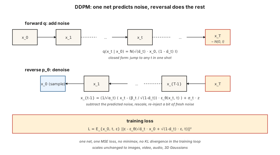
Forward process q. Add Gaussian noise in T small steps. The closed form — the reason the math is tractable — is that the cumulative step is also Gaussian:
where \bar\alpha_t = \prod_{s=1}^{t} (1 - \beta_s) for a schedule of \beta_t. Pick \beta_t from 1e-4 to 0.02 linearly over T=1000 steps and x_T is approximately \mathcal{N}(0, I).
Reverse process p_\theta. Learn a neural net \epsilon_\theta(x_t, t) that predicts the noise that was added. Given x_t, denoise by:
where \sigma_t is either \sqrt{\beta_t} or a learned variance. The expression is ugly but it is just algebra — solving for x_{t-1} given the posterior q(x_{t-1} \mid x_t, x_0) and substituting x_0 with its noise-predicted estimate.
Training loss.
Sample x_0 from data, pick a random t, sample \epsilon \sim \mathcal{N}(0, I), compute the noisy x_t in one shot via the closed form, and regress on the noise. One loss, no minimax, no KL, no reparameterization tricks.
Sampling. Start x_T \sim \mathcal{N}(0, I). Iterate the reverse step from t = T to 1. Done.
Why it works
Three intuitions:
- Denoising is easy; generating is hard. At t=T, the data is pure noise — the net has to solve a trivial problem. At t=0, the net only has to clean up a few pixels. At intermediate t, the problem is hard but the net has many gradients flowing through the same weights from every noise level.
- Score matching in disguise. Vincent (2011) proved that predicting the noise is equivalent to estimating \nabla_x \log q(x_t \mid x_0), the score. The reverse SDE uses this score to walk up the density gradient — a guided random walk toward high-probability regions.
- The ELBO reduces to simple MSE. The full variational lower bound has a KL term per timestep. With DDPM's parameterization those KL terms simplify to MSE on noise prediction with specific coefficients; Ho dropped the coefficients (calling it "simple" loss) and quality improved.
Build It
code/main.py implements a 1-D DDPM. Data is a two-mode mixture. The "net" is a tiny MLP that takes (x_t, t) and outputs predicted noise. Training is the one-line loss. Sampling iterates the reverse chain.
Step 1: the forward schedule (closed form)
pythonbetas = [1e-4 + (0.02 - 1e-4) * t / (T - 1) for t in range(T)]
alphas = [1 - b for b in betas]
alpha_bars = []
cum = 1.0
for a in alphas:
cum *= a
alpha_bars.append(cum)Step 2: sample x_t in one shot
pythondef forward_sample(x0, t, alpha_bars, rng):
a_bar = alpha_bars[t]
eps = rng.gauss(0, 1)
x_t = math.sqrt(a_bar) * x0 + math.sqrt(1 - a_bar) * eps
return x_t, epsStep 3: one training step
pythondef train_step(x0, model, alpha_bars, rng):
t = rng.randrange(T)
x_t, eps = forward_sample(x0, t, alpha_bars, rng)
eps_hat = model_forward(model, x_t, t)
loss = (eps - eps_hat) ** 2
return loss, gradient_step(model, ...)Step 4: reverse sampling
pythondef sample(model, alpha_bars, T, rng):
x = rng.gauss(0, 1)
for t in range(T - 1, -1, -1):
eps_hat = model_forward(model, x, t)
beta_t = 1 - alphas[t]
x = (x - beta_t / math.sqrt(1 - alpha_bars[t]) * eps_hat) / math.sqrt(alphas[t])
if t > 0:
x += math.sqrt(beta_t) * rng.gauss(0, 1)
return xFor a 1-D problem with 40 timesteps and a 24-unit MLP, this learns the two-mode mixture in ~200 epochs.
Time conditioning
The net needs to know which timestep it is denoising. Two standard options:
- Sinusoidal embedding. Like Transformer positional encoding. \text{embed}(t) = [\sin(t/\omega_0), \cos(t/\omega_0), \sin(t/\omega_1), \ldots]. Pass through an MLP, broadcast into the net.
- Film / group-norm conditioning. Project embedding to per-channel scale/bias (FiLM) at each block.
Our toy code uses sinusoidal → concat. Production U-Nets use FiLM.
Pitfalls
- Schedule matters a lot. Linear \beta is the DDPM default but cosine schedule (Nichol & Dhariwal, 2021) gives better FID for the same compute. Switch schedules if quality plateaus.
- Timestep embedding is fragile. Passing raw t as a float works for toy 1-D but fails for images; always use a proper embedding.
- V-prediction vs ε-prediction. For narrow regimes (very small or very large t), \epsilon has poor signal-to-noise. V-prediction (v = \alpha \cdot \epsilon - \sigma \cdot x) is more stable; SDXL, SD3, and Flux use it.
- Classifier-free guidance. At inference, compute both conditional and unconditional \epsilon, then \epsilon_{\text{cfg}} = (1 + w) \cdot \epsilon_{\text{cond}} - w \cdot \epsilon_{\text{uncond}} with w \approx 3\text{-}7. Covered in Lesson 08.
- 1000 steps is a lot. Production uses DDIM (20-50 steps), DPM-Solver (10-20 steps), or distillation (1-4 steps). See Lesson 12.
Use It
| Role | Typical stack in 2026 |
|---|---|
| Image pixel-space diffusion (small, toy) | DDPM + U-Net |
| Image latent diffusion | VAE encoder + U-Net or DiT (Lesson 07) |
| Video latent diffusion | Spatiotemporal DiT (Sora, Veo, WAN) |
| Audio latent diffusion | Encodec + diffusion transformer |
| Science (molecules, proteins, physics) | Equivariant diffusion (EDM, RFdiffusion, AlphaFold3) |
Diffusion is the universal generative backbone. Flow matching (Lesson 13) is the 2024-2026 competitor that usually wins on inference speed for the same quality.
Ship It
Save outputs/skill-diffusion-trainer.md. Skill takes a dataset + compute budget and outputs: schedule (linear/cosine/sigmoid), prediction target (ε/v/x), number of steps, guidance scale, sampler family, and an eval protocol.
Exercises
- Easy. Change T from 40 to 10 in
code/main.py. How does sample quality (visual histogram of outputs) degrade? At what T does the two-mode structure collapse? - Medium. Switch from ε-prediction to v-prediction. Re-derive the reverse step. Compare final sample quality.
- Hard. Add classifier-free guidance. Condition on a class label c \in \lbrace 0, 1 \rbrace, drop it 10% of the time during training, and at sampling time use \epsilon = (1+w) \cdot \epsilon_{\text{cond}} - w \cdot \epsilon_{\text{uncond}}. Measure the conditional-mode-hit rate at w = 0, 1, 3, 7.
Key Terms
| Term | What people say | What it actually means |
|---|---|---|
| Forward process | "Adding noise" | Fixed Markov chain q(x_t \mid x_{t-1}) that destroys the data. |
| Reverse process | "Denoising" | Learned chain p_\theta(x_{t-1} \mid x_t) that reconstructs the data. |
| β schedule | "The noise ladder" | Per-step variance; linear, cosine, or sigmoid. |
| α̅ | "Alpha bar" | Cumulative product \prod (1 - \beta); gives closed-form x_t from x_0. |
| Simple loss | "MSE on noise" | \lVert \epsilon - \epsilon_\theta(x_t, t) \rVert^2; all variational derivations collapse to this. |
| ε-prediction | "Predict noise" | Output is the noise added; standard DDPM. |
| V-prediction | "Predict velocity" | Output is \alpha \cdot \epsilon - \sigma \cdot x; better conditioning across t. |
| DDPM | "The paper" | Ho et al. 2020; linear β, 1000 steps, U-Net. |
| DDIM | "Deterministic sampler" | Non-Markov sampler, 20-50 steps, same training objective. |
| Classifier-free guidance | "CFG" | Mix conditional and unconditional noise predictions to amplify conditioning. |
Production note: diffusion inference is a step-count problem
The DDPM paper runs T=1000 reverse steps. Nobody ships that in production. Every real inference stack picks one of three strategies — and each maps cleanly to production framing of "where is the latency coming from":
- Faster sampler, same model. DDIM (20-50 steps), DPM-Solver++ (10-20), UniPC (8-16). Drop-in replacement of the reverse loop; the trained \epsilon_\theta weights are untouched. Cuts latency 20-50×.
- Distillation. Train a student to match the teacher in fewer steps: Progressive Distillation (2 → 1), Consistency Models (arbitrary → 1-4), LCM, SDXL-Turbo, SD3-Turbo. Cuts latency another 5-10×, requires retraining.
- Caching and compilation.
torch.compile(unet, mode="reduce-overhead"), TensorRT-LLM's diffusion backends,xformers/SDPA attention, bf16 weights. Cuts per-step latency ~2×. Stacks with (1) and (2).
For a production diffusion server the budget conversation is the same as production literature describes for LLMs: latency is num_steps × step_cost + VAE_decode, throughput is batch_size × (num_steps × step_cost)^-1. TTFT is small (one step); TPOT-equivalent is the full response time because image generation is "all-at-once" from the user's perspective.
Further Reading
- Sohl-Dickstein et al. (2015). Deep Unsupervised Learning using Nonequilibrium Thermodynamics — the diffusion paper, ahead of its time.
- Ho, Jain, Abbeel (2020). Denoising Diffusion Probabilistic Models — DDPM.
- Song, Meng, Ermon (2021). Denoising Diffusion Implicit Models — DDIM, fewer steps.
- Nichol & Dhariwal (2021). Improved DDPM — cosine schedule, learned variance.
- Dhariwal & Nichol (2021). Diffusion Models Beat GANs on Image Synthesis — classifier guidance.
- Ho & Salimans (2022). Classifier-Free Diffusion Guidance — CFG.
- Karras et al. (2022). Elucidating the Design Space of Diffusion-Based Generative Models (EDM) — unified notation, cleanest recipe.
Diagrams1 figure