问题
"The food was not great." 是正面还是负面?
情感分析听起来简单:评论者说喜欢或不喜欢某样东西,给句子打个标签。它之所以成为最经典的 NLP 任务,是因为每个看起来简单的例子背后都藏着一个难的。否定会翻转含义,讽刺会把它倒过来,"Not bad at all" 明明是正面却包含两个负面编码词。表情符号携带的信号可能比 surrounding text 还多。领域词汇也很重要(tight 在音乐评论里 vs 时尚评论里)。
情感分析是经典 NLP 的绝佳实验室。如果你理解为什么每个朴素基线都有特定的失效模式,你就能理解为什么每个更复杂的模型会被发明出来。本节课从零构建 Naive Bayes 基线,加入 logistic 回归,并指出让生产级情感分析变成合规级问题的那些陷阱。
概念
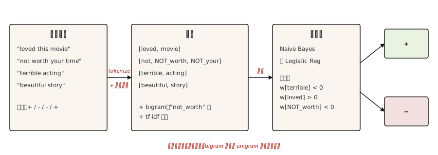
经典情感分析是一个两步配方:
- 表示。 把文本变成特征向量。BoW、TF-IDF 或 n-gram。
- 分类。 在带标签样本上拟合线性模型(Naive Bayes、logistic 回归、SVM)。
Naive Bayes 是最蠢但有效的模型。假设每个特征在给定标签下条件独立。从计数中估计 P(word | positive) 和 P(word | negative)。推理时把概率相乘。"朴素"的独立性假设错得可笑,结果却强得惊人。原因是:文本特征稀疏、数据量中等时,分类器更关心每个词倾向哪一边,而不是词与词之间的依赖。
Logistic 回归修正了独立性假设。它学习每个特征的权重,包括负权重。not good 作为二元组特征会得到负权重,而 Naive Bayes 对它从未标注过的二元组做不到这一点。
构建它
第 1 步:一个真实的微型数据集
pythonPOSITIVE = [
"absolutely loved this movie",
"beautiful cinematography and a great story",
"one of the best films of the year",
"brilliant acting from the lead",
"heartwarming and funny",
]
NEGATIVE = [
"boring and far too long",
"not worth your time",
"the plot made no sense",
"terrible acting, awful script",
"i want my two hours back",
]故意弄得很小。真实工作会用数万个样本(IMDb、SST-2、Yelp polarity)。数学是一样的。
第 2 步:从零开始的多项式 Naive Bayes
pythonimport math
from collections import Counter
def train_nb(docs_by_class, vocab, alpha=1.0):
class_priors = {}
class_word_probs = {}
total_docs = sum(len(d) for d in docs_by_class.values())
for cls, docs in docs_by_class.items():
class_priors[cls] = len(docs) / total_docs
counts = Counter()
for doc in docs:
for token in doc:
counts[token] += 1
total = sum(counts.values()) + alpha * len(vocab)
class_word_probs[cls] = {
w: (counts[w] + alpha) / total for w in vocab
}
return class_priors, class_word_probs
def predict_nb(doc, class_priors, class_word_probs):
scores = {}
for cls in class_priors:
s = math.log(class_priors[cls])
for token in doc:
if token in class_word_probs[cls]:
s += math.log(class_word_probs[cls][token])
scores[cls] = s
return max(scores, key=scores.get)加法平滑(alpha=1.0)就是 Laplace 平滑。没有它,某个词在某个类里未出现时概率为零,log 会爆炸。实践中常用 alpha=0.01;alpha=1.0 是教学默认值。
第 3 步:从零开始的 Logistic 回归
pythonimport numpy as np
def sigmoid(x):
return 1.0 / (1.0 + np.exp(-np.clip(x, -20, 20)))
def train_lr(X, y, epochs=500, lr=0.05, l2=0.01):
n_features = X.shape[1]
w = np.zeros(n_features)
b = 0.0
for _ in range(epochs):
logits = X @ w + b
preds = sigmoid(logits)
err = preds - y
grad_w = X.T @ err / len(y) + l2 * w
grad_b = err.mean()
w -= lr * grad_w
b -= lr * grad_b
return w, b
def predict_lr(X, w, b):
return (sigmoid(X @ w + b) >= 0.5).astype(int)L2 正则化在这里很重要。文本特征稀疏,没有 L2 模型会记住训练样本。从 0.01 开始调参。
第 4 步:处理否定(失效模式)
看 "not good" 和 "not bad"。BoW 分类器看到 {not, good} 和 {not, bad},只能从训练集中哪个出现更多来学习。二元组分类器看到 not_good 和 not_bad,把它们当成不同特征,这通常就够了。
没有二元组时也能用的粗糙但有效的方法:否定作用域(negation scoping)。在否定词之后、遇到下一个标点之前,给每个 token 加上 NOT_ 前缀。
pythonNEGATION_WORDS = {"not", "no", "never", "nor", "none", "nothing", "neither"}
NEGATION_TERMINATORS = {".", "!", "?", ",", ";"}
def apply_negation(tokens):
out = []
negate = False
for token in tokens:
if token in NEGATION_TERMINATORS:
negate = False
out.append(token)
continue
if token in NEGATION_WORDS:
negate = True
out.append(token)
continue
out.append(f"NOT_{token}" if negate else token)
return outpython>>> apply_negation(["not", "good", "at", "all", ".", "but", "funny"])
['not', 'NOT_good', 'NOT_at', 'NOT_all', '.', 'but', 'funny']现在 good 和 NOT_good 是不同的特征,分类器可以给它们相反的权重。三行预处理,能在情感基准上带来可测量的准确率提升。
第 5 步:真正重要的评估指标
类别不平衡时,只看准确率会误导。真实情感语料通常是 70-80% 正面或 70-80% 负面;一个永远预测多数类的分类器能得到 80% 准确率,却毫无价值。以下每一项都要报告:
- 每类精确率与召回率。 每类一对,再 macro-average 成一个尊重类别平衡的单一数字。
- Macro-F1(不平衡数据的首要指标)。 每类 F1 的平均值,等权重。类别不平衡时用它代替准确率。
- Weighted-F1(替代指标)。 与 macro-F1 相同,但按类别频率加权。当不平衡本身有业务含义时一并报告。
- 混淆矩阵。 原始计数。在相信任何标量指标之前都要先看它;它能揭示模型把哪两类搞混。
- 每类错误样本。 每类抽 5 个错误预测,读一遍。没有什么能替代读真实错误。
严重不平衡数据(比例 > 95:5)要报告 AUROC 和 AUPRC。AUPRC 对少数类更敏感,而少数类通常才是你真正关心的(垃圾邮件、欺诈、罕见情感)。
要避免的常见错误。 在不平衡数据上报告 micro-F1 会得到一个看起来很高的数字,因为它被多数类主导。Macro-F1 强迫你看到少数类表现。
pythondef evaluate(y_true, y_pred):
tp = sum(1 for t, p in zip(y_true, y_pred) if t == 1 and p == 1)
fp = sum(1 for t, p in zip(y_true, y_pred) if t == 0 and p == 1)
fn = sum(1 for t, p in zip(y_true, y_pred) if t == 1 and p == 0)
tn = sum(1 for t, p in zip(y_true, y_pred) if t == 0 and p == 0)
precision = tp / (tp + fp) if tp + fp else 0
recall = tp / (tp + fn) if tp + fn else 0
f1 = 2 * precision * recall / (precision + recall) if precision + recall else 0
return {"tp": tp, "fp": fp, "tn": tn, "fn": fn, "precision": precision, "recall": recall, "f1": f1}使用它
scikit-learn 用六行就能正确实现。
pythonfrom sklearn.feature_extraction.text import TfidfVectorizer
from sklearn.linear_model import LogisticRegression
from sklearn.pipeline import Pipeline
pipe = Pipeline([
("tfidf", TfidfVectorizer(ngram_range=(1, 2), min_df=2, sublinear_tf=True, stop_words=None)),
("clf", LogisticRegression(C=1.0, max_iter=1000)),
])
pipe.fit(X_train, y_train)
print(pipe.score(X_test, y_test))注意三件事。stop_words=None 保留否定词;ngram_range=(1, 2) 加入二元组,让 not_good 成为特征;sublinear_tf=True 压低重复词的权重。这三个开关就是 SST-2 上 75% 准确率基线和 85% 准确率基线之间的差距。
何时该上 Transformer
- 讽刺检测。经典模型在这里必败。
- 长评论,情感在文档中途转变。
- 基于方面的情感分析。"Camera was great but battery was terrible." 你需要把情感归因到具体方面,只有 Transformer 或结构化输出模型才能做到。
- 非英语、低资源语言。多语言 BERT 能免费提供零样本基线。
如果你需要以上任何一种,跳到第 7 阶段(Transformer 深入剖析)。否则,TF-IDF + 二元组 + 否定处理上的 Naive Bayes 或 logistic 回归就是你在 2026 年的生产基线。
可复现性陷阱(再次出现)
重新训练情感模型是常规操作,重新评估却不是。论文里报告的准确率数字来自特定的划分、特定的预处理、特定的 tokenizer。如果你不用完全相同的管道去比较新模型和基线,就会得到误导性的差距。总是要在你的管道上重新生成基线,而不是直接引用论文数字。
交付它
保存为 outputs/prompt-sentiment-baseline.md:
markdown---
name: sentiment-baseline
description: Design a sentiment analysis baseline for a new dataset.
phase: 5
lesson: 05
---
Given a dataset description (domain, language, size, label granularity, latency budget), you output:
1. Feature extraction recipe. Specify tokenizer, n-gram range, stopword policy (usually keep), negation handling (scoped prefix or bigrams).
2. Classifier. Naive Bayes for baseline, logistic regression for production, transformer only if the domain needs sarcasm / aspects / cross-lingual.
3. Evaluation plan. Report precision, recall, F1, confusion matrix, and per-class error samples (not just scalars).
4. One failure mode to monitor post-deployment. Domain drift and sarcasm are the top two.
Refuse to recommend dropping stopwords for sentiment tasks. Refuse to report accuracy as the sole metric when classes are imbalanced (e.g., 90% positive). Flag subword-rich languages as needing FastText or transformer embeddings over word-level TF-IDF.练习
- 简单。 把
apply_negation作为预处理步骤加入 scikit-learn 管道,在一个小型情感数据集上测量 F1 提升。 - 中等。 实现类别加权 logistic 回归(把
class_weight="balanced"传给 scikit-learn,或自己推导梯度)。测量在合成 90:10 类别不平衡上的效果。 - 困难。 通过对情感模型残差训练第二个分类器,构建一个讽刺检测器。记录实验设置。当准确率低于随机水平时警告读者(二分类讽刺检测的随机水平约 50%,大多数第一次尝试都会落在那里)。
关键术语
| 术语 | 人们的说法 | 实际含义 |
|---|---|---|
| Polarity | 正面或负面 | 二分类标签;有时会扩展为中性或细粒度(5 星)。 |
| Aspect-based sentiment | 按方面极性 | 把情感归因到文本中提到的具体实体或属性。 |
| Negation scoping | 反转附近 token | 在 "not" 之后、遇到标点前,给 token 加上 NOT_ 前缀。 |
| Laplace smoothing | 计数加 1 | 防止 Naive Bayes 中出现零概率特征。 |
| L2 regularization | 收缩权重 | 在损失中加入 lambda * sum(w^2)。对稀疏文本特征至关重要。 |
延伸阅读
- Pang and Lee (2008). Opinion Mining and Sentiment Analysis —— 奠基性综述。很长,但前四节覆盖了所有经典内容。
- Wang and Manning (2012). Baselines and Bigrams: Simple, Good Sentiment and Topic Classification —— 这篇论文证明了二元组 + Naive Bayes 在短文本上很难被打败。
- scikit-learn text feature extraction docs ——
CountVectorizer、TfidfVectorizer以及你要调的每个参数的参考。
示意图共 1 张